Regression

When you analyse experimental data you will want to see whether there is any relation between the sets of data. One way to do this is to calculate the Pearson product-moment correlation coefficient.

Pearson's Product-Moment Correlation Coefficient

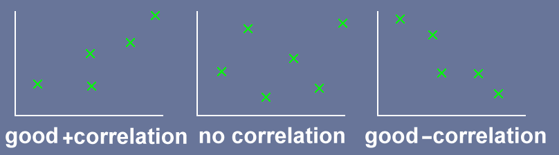
Karl Pearson devised a coefficient to measure the correlation between two sets of data. The coefficient ranges from $-1$ to $1$. A value of $1$ means there is perfect correlation between the data sets, a value of $0$ means there is no correlation and a value of $-1$ means there is perfect negative correlation between the data sets. Note: independent data may be strongly correlated, correlation does not mean causality. Have a look at Tyler Vigen's Spurious Correlations

Assume you have a set of independent data, $x$, with corresponding dependent data, $y$, then Pearson's product-moment correlation coefficient is given by:

If $|r| \geq 0.5$ then you will want to find the gradient and y-intercept of the regression line. To do this we will use the method of least squares. Least squares minimises the square of the perpendicular distance between each data point and the regression line. The square of the distance is used because points below the line give a negative distance and we want to minimise to sum of all the separate distances. The gradient and y-intercept are given by:

Finally, we need to think about the units of the gradient and y-intercept. The y-intercept has the same units as $y$. The gradient is the rate of change of $y$ divided by the rate of change of $x$. If $x$ was measured in seconds and $y$ was measured in metres then the gradient would be measured in metres per second (m/s or ms^-1).

Example 1: Given the following data calculate the Pearson correlation coefficient. $x$ is measured in seconds and $y$ is measured in degrees kelvin.

$x$ (s)	0	1	2	3	4
$y$ (K)	8	14	13	20	19

To find $r$ we need $\sum x$, $\sum y$, $\sum xy$, $\sum x^2$, $\sum y^2$ and $n$.

$x$	0	1	2	3	4	10
$y$	8	14	13	20	19	74
$xy$	0	14	26	60	76	176
$x^2$	0	1	4	9	16	30
$y^2$	64	196	169	400	361	1190

Putting these values into Pearson's equation

$r=\frac{n \sum xy- \sum x \sum y}{\sqrt{n\sum x^2-(\sum x)^2} \times \sqrt{n\sum y^2-(\sum y)^2}}$

$=\frac{5 \times 176 - 10 \times 74}{\sqrt{5 \times 30 - 10^2} \times \sqrt{5 \times 1190 - 74^2}}$

$=0.909$

A value for $r=0.909$ means there is a high correlation for these data which means it is worth calculating the gradient and y-intercept of the correlation line.

$m=\frac{n \sum xy- \sum x \sum y}{n\sum x^2-(\sum x)^2}$

$=\frac{5 \times 176 - 10 \times 74}{5 \times 30 - 10^2}$

$=2.80$ K/s

$c=\frac{ \sum x^2 \times \sum y - \sum x \sum xy}{n\sum x^2-(\sum x)^2} $

$=\frac{30 \times 74 - 10 \times 176}{5 \times 30 - 10^2}$

$=9.2$ K

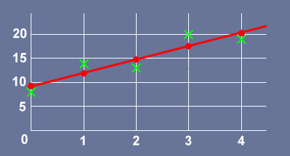
Here is a plot of the data and the regression line